Advanced Quantum Kernel Methods

Introduction

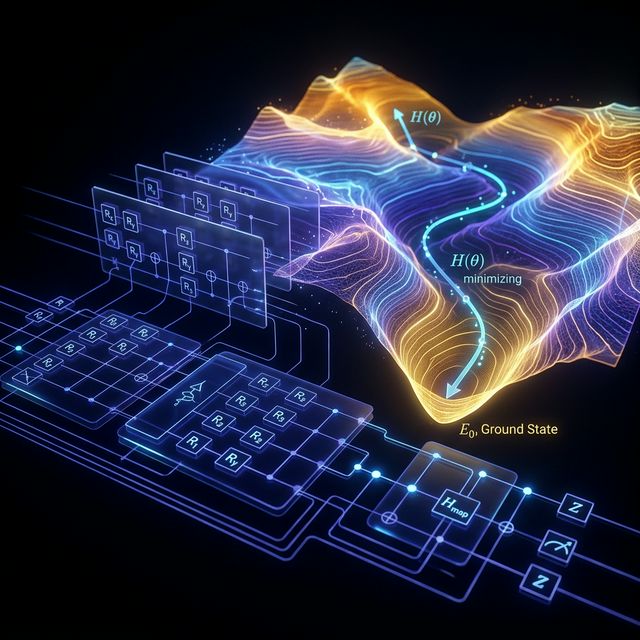
Quantum kernel methods represent one of the most theoretically grounded approaches to quantum machine learning. Unlike variational quantum circuits, which suffer from barren plateaus and trainability issues (see our article on QNN convergence), kernel methods shift the quantum computation to a fixed subroutine — the kernel evaluation — while the learning algorithm remains entirely classical.

The key idea: use a quantum circuit as a feature map that embeds classical data into an exponentially large Hilbert space, then compute inner products in that space as a kernel function for classical algorithms like Support Vector Machines.

This article derives the full mathematical framework from scratch.

1. Classical Kernel Methods: The Foundation

Before introducing quantum kernels, we need to be precise about what a kernel is.

1.1 The Kernel Trick

Given a dataset $\{(x_i, y_i)\}_{i=1}^m$ with $x_i \in \mathcal{X}$ and $y_i \in \{-1, +1\}$ , a kernel function is a symmetric positive semi-definite function:

k: \mathcal{X} \times \mathcal{X} \to \mathbb{R}, \quad k(x, x') = \langle \phi(x), \phi(x') \rangle_{\mathcal{H}}

where $\phi: \mathcal{X} \to \mathcal{H}$ is a feature map into a Hilbert space $\mathcal{H}$ (which may be infinite-dimensional), and $\langle \cdot, \cdot \rangle_{\mathcal{H}}$ is the inner product in $\mathcal{H}$ .

By Mercer’s theorem, any continuous positive semi-definite function on a compact domain is a valid kernel corresponding to some feature map. This means we never need to explicitly compute $\phi(x)$ — only the pairwise inner products $k(x_i, x_j)$ .

1.2 The SVM Primal Problem

The hard-margin SVM finds the maximum-margin hyperplane in $\mathcal{H}$ :

\min_{w \in \mathcal{H},\, b \in \mathbb{R}} \frac{1}{2}\|w\|_{\mathcal{H}}^2 \quad \text{subject to} \quad y_i(\langle w, \phi(x_i)\rangle_{\mathcal{H}} + b) \geq 1 \;\; \forall i

1.3 The Dual Problem

By the KKT conditions, the dual problem depends only on inner products:

\max_{\alpha \geq 0} \sum_{i=1}^{m} \alpha_i - \frac{1}{2}\sum_{i,j=1}^{m} \alpha_i \alpha_j y_i y_j k(x_i, x_j)

subject to $\sum_i \alpha_i y_i = 0$ . The decision function is:

f(x) = \text{sign}\!\left(\sum_{i=1}^{m} \alpha_i y_i k(x_i, x) + b\right)

This is entirely computable from the kernel matrix $K_{ij} = k(x_i, x_j)$ without ever explicitly constructing $\phi(x)$ . This is the kernel trick.

2. Quantum Feature Maps

2.1 Definition

A quantum feature map $\Phi: \mathbb{R}^d \to \mathcal{B}(\mathcal{H}_n)$ maps classical data $x \in \mathbb{R}^d$ to a density matrix in the space of bounded operators on an $n$ -qubit Hilbert space $\mathcal{H}_n = (\mathbb{C}^2)^{\otimes n}$ :

\Phi(x) = U_\phi(x)|0\rangle\langle 0|^{\otimes n} U_\phi^\dagger(x) = |\phi(x)\rangle\langle\phi(x)|

where $U_\phi(x)$ is a parameterized unitary circuit that depends on the data point $x$ .

The quantum state $|\phi(x)\rangle = U_\phi(x)|0\rangle^{\otimes n}$ lives in a Hilbert space of dimension $2^n$ — exponentially large in the number of qubits.

2.2 The Quantum Kernel Function

The quantum kernel is defined as the squared overlap (fidelity) between two quantum feature states:

k_Q(x, x') = |\langle \phi(x) | \phi(x') \rangle|^2 = \left|\langle 0|^{\otimes n} U_\phi^\dagger(x) U_\phi(x') |0\rangle^{\otimes n}\right|^2

This is exactly the probability of measuring the all-zeros bitstring $|0\rangle^{\otimes n}$ after running the circuit $U_\phi^\dagger(x) U_\phi(x')$ on the zero state.

This is directly measurable on quantum hardware. No classical post-processing of exponentially large vectors is required — the kernel value is a measurement probability.

2.3 Positive Semi-Definiteness

The quantum kernel is a valid kernel function. Proof: The kernel matrix $K$ with entries $K_{ij} = k_Q(x_i, x_j)$ is positive semi-definite because:

K_{ij} = \text{Tr}[\Phi(x_i)\Phi(x_j)] = \langle \Phi(x_i), \Phi(x_j) \rangle_{\text{HS}}

where $\langle A, B \rangle_{\text{HS}} = \text{Tr}[A^\dagger B]$ is the Hilbert-Schmidt inner product. This is an inner product on the space of density matrices, so $K$ is positive semi-definite by construction. $\square$

3. The IQP Feature Map (Havlíček et al., 2019)

The landmark paper by Havlíček et al. [2019, Nature] introduced a specific quantum feature map based on Instantaneous Quantum Polynomial (IQP) circuits and argued that the corresponding kernel is classically hard to estimate.

3.1 Circuit Construction

For $n$ qubits and input $x \in \mathbb{R}^n$ , the feature map circuit is:

U_\phi(x) = \left(\prod_{S \subseteq [n]} e^{i\phi_S(x)Z_S}\right) H^{\otimes n} \left(\prod_{S \subseteq [n]} e^{i\phi_S(x)Z_S}\right) H^{\otimes n}

The circuit applies two rounds of Hadamard gates interleaved with diagonal unitaries. The phase functions are:

\phi_{\{i\}}(x) = x_i, \quad \phi_{\{i,j\}}(x) = (\pi - x_i)(\pi - x_j)

where in practice only nearest-neighbor and next-nearest-neighbor pairs $\{i,j\}$ are included to keep the circuit implementable on hardware with limited connectivity.

3.2 Classical Hardness Argument

Havlíček et al. argue (with caveats) that classically simulating this kernel efficiently would imply a collapse of the polynomial hierarchy. Specifically, estimating $k_Q(x, x')$ to within additive error $1/\text{poly}(n)$ in polynomial time classically would require solving problems in $\#\text{P}$ efficiently, which is believed impossible.

Important caveat: This hardness is for worst-case inputs, not necessarily the data distributions encountered in practice. Whether this hardness translates to practical learning advantage remains an open and actively debated question [Schuld & Killoran, 2022; Huang et al., 2021].

4. The Kernel Matrix and Quantum Advantage

4.1 Computing the Full Kernel Matrix

For a training set of $m$ examples, computing the full kernel matrix $K \in \mathbb{R}^{m \times m}$ requires $O(m^2)$ quantum circuit evaluations. Each evaluation runs the circuit $U_\phi^\dagger(x_i)U_\phi(x_j)$ and measures in the computational basis, with the kernel value estimated as the frequency of the $|0\rangle^{\otimes n}$ outcome over $T$ shots:

\hat{k}_Q(x_i, x_j) = \frac{\text{count}(|0\rangle^{\otimes n})}{T}

Statistical error in this estimate is $O(1/\sqrt{T})$ by the central limit theorem. For $\epsilon$ -accurate kernel estimation, we need $T = O(1/\epsilon^2)$ shots per entry.

4.2 When Can Quantum Kernels Win?

Huang et al. [2021, Nature Communications] proved a rigorous separation result: there exist learning problems for which:

\text{Error}(k_Q) = O\left(\frac{1}{m}\right), \quad \text{Error}(k_{\text{classical}}) = \Omega(1)

for any classical kernel in a fixed class, given $m$ training examples. The constructed problem involves learning properties of quantum processes — not a natural classical ML problem, but a genuine provable advantage.

For classical data distributions, the picture is murkier. The quantum kernel must access features that are hard to compute classically for a genuine advantage. If the relevant features are easy to compute classically, then a classical kernel can match quantum performance [Schuld & Killoran, 2022, Physical Review Letters].

4.3 The Geometric Difference

Liu et al. [2021, Nature Physics] quantified the relationship between classical and quantum kernels via the geometric difference:

g(k_Q, k_c) = \sqrt{\left\|\sqrt{K_Q} K_c^{-1} \sqrt{K_Q}\right\|_\infty}

where $K_Q$ and $K_c$ are the quantum and classical kernel matrices. When $g$ is large, the quantum kernel captures features that the classical kernel misses. Quantum advantage in generalization scales with $g$ .

5. Practical Considerations

5.1 Kernel Alignment

Not all quantum feature maps are useful. A feature map is well-suited to a task when the corresponding kernel has high target alignment:

A(K, y) = \frac{\langle K, yy^T \rangle_F}{\|K\|_F \|yy^T\|_F}

where $y = (y_1, \ldots, y_m)^T$ is the label vector and $\langle \cdot, \cdot \rangle_F$ is the Frobenius inner product. High alignment means the kernel matrix naturally clusters data by class label. One can use this as a guide to design or select quantum feature maps before training.

5.2 Number of Qubits vs. Feature Dimension

For $n$ qubits, the feature space dimension is $2^n$ . This means:

Qubits ( $n$ )	Feature space dim.	Classical equivalent
10	1,024	Feasible classically
20	1,048,576	Hard but not impossible
50	$\approx 10^{15}$	Far beyond classical
100	$\approx 10^{30}$	Classically intractable

However, not all $2^n$ dimensions are necessarily useful for a given learning problem. The intrinsic dimensionality of the learning problem may be much lower.

5.3 Shot Noise and Sample Complexity

A significant practical challenge: to estimate a single kernel entry to accuracy $\epsilon$ , we need $O(1/\epsilon^2)$ shots. For a training set of $m = 1000$ examples, the full kernel matrix has $m(m+1)/2 \approx 500{,}000$ unique entries. At $T = 1000$ shots per entry, this requires $5 \times 10^8$ circuit executions. On current hardware running at $\sim 10^3$ circuits/second, this takes roughly $5 \times 10^5$ seconds — far from practical.

This is a genuine bottleneck that current research is working to address via kernel approximation methods and more efficient circuit designs.

6. Current Status and Open Questions

The field of quantum kernels is active and honest about its limitations:

Established:

Quantum kernels are valid kernel functions with quantum circuit estimation procedures [Havlíček et al., 2019]
Provable learning advantage exists for specifically constructed quantum tasks [Huang et al., 2021]
Kernel alignment provides a trainable way to optimize feature maps [Hubregtsen et al., 2022, Quantum Machine Intelligence]

Open:

Whether quantum kernels provide advantage on practically relevant classical datasets
How to design feature maps that balance expressibility with circuit depth constraints
Efficient estimation methods that reduce the $O(m^2/\epsilon^2)$ shot requirement

Conclusion

Quantum kernel methods are one of the most mathematically rigorous approaches in quantum ML. They avoid the barren plateau problem entirely and connect directly to well-understood classical learning theory. The quantum speedup, where it exists, comes from the hardness of classically simulating the quantum feature map.

The honest assessment: they are the right way to think about near-term quantum ML for classification tasks, but practical advantage on real classical datasets has not yet been demonstrated. That is the frontier. The mathematics is correct; the engineering challenge remains.

References

Havlíček, V., Córcoles, A. D., Temme, K., Harrow, A. W., Kandala, A., Chow, J. M., & Gambetta, J. M. (2019). Supervised learning with quantum-enhanced feature spaces. Nature, 567(7747), 209–212. https://doi.org/10.1038/s41586-019-0980-2
Huang, H.-Y., Broughton, M., Mohseni, M., Babbush, R., Boixo, S., Neven, H., & McClean, J. R. (2021). Power of data in quantum machine learning. Nature Communications, 12(1), 2631. https://doi.org/10.1038/s41467-021-22539-9
Schuld, M., & Killoran, N. (2022). Is quantum advantage the right goal for quantum machine learning? PRX Quantum, 3(3), 030101. https://doi.org/10.1103/PRXQuantum.3.030101
Liu, Y., Arunachalam, S., & Temme, K. (2021). A rigorous and robust quantum speed-up in supervised machine learning. Nature Physics, 17(9), 1013–1017. https://doi.org/10.1038/s41567-021-01287-z
Hubregtsen, T., Wierichs, D., Gil-Fuster, E., Derks, P.-J. H. S., Faehrmann, P. K., & Meyer, J. J. (2022). Training quantum embedding kernels on near-term quantum computers. Quantum Machine Intelligence, 4(1), 6. https://doi.org/10.1007/s42484-022-00060-6
Schuld, M. (2021). Supervised quantum machine learning models are kernel methods. arXiv preprint arXiv:2101.11020. https://arxiv.org/abs/2101.11020

#quantum kernels #SVM #feature maps #quantum advantage #RKHS #quantum ML

Rashan is a Data Science Professional and Quantum AI Researcher, and the Founder & CEO of Intellit — an AI automation agency building intelligent systems across fintech, banking, and enterprise sectors.

The Quantum Intelligence Digest

Join researchers and engineers who read Quaniq.